Enumerating some solutions for those Manhattan distance problems

Continued from “Étude: How much do you need to know?” and “More on inferring lattice position from Manhattan distances”.

Reviewing

The other day I framed an étude about how much information (and to some extent, which information) you need to know, to be 100% confident that your solution to a simple numerical assignment problem is “correct”.

We started off by talking about arbitrary square arrangements of labeled positions in a square lattice: Given the numbers 1 through 9 arranged in a 3x3 square, and given a list of all the Manhattan distances between all 36 pairs of numbers, I suggested that you could be 100% certain that the arrangement of the numbers’ positions, except for rotation and reflection symmetry.

So for example, suppose the “right answer” is this square:

 1  2  3
 4  5  6
 7  8  9

When I tell you the Manhattan distances between all pairs of numbers ([1,2], [1,3], [1,4] and so on up to [8,9]), then the only arrangements of those nine numbers that are consistent with all 36 distance “clues” are these eight:

 1  2  3    7  4  1    9  8  7    3  6  9
 4  5  6    8  5  2    6  5  4    2  5  8
 7  8  9    9  6  3    3  2  1    1  4  7

 3  2  1    9  6  3    7  8  9    1  4  7   
 6  5  4    8  5  2    4  5  6    2  5  8   
 9  8  7    7  4  1    1  2  3    3  6  9    

Assuming that I’ve rotated and flipped these correctly as I typed them in, you should be able to see that they’re reflected across the horizontal axis, and each step to the right rotates a square clockwise. That’s what I was going for, at least.

Actually, as I write this, I realize there’s no particular reason these labels need to be numeric. I could use anything at all to differentiate positions: colors, symbols, whatever I want as long as they’re all unique. Let’s switch to letters for a minute. These are the same eight solutions I showed above, but with letters:

 A  B  C    G  D  A    I  H  G    C  F  I
 D  E  F    H  E  B    F  E  D    B  E  H
 G  H  I    I  F  C    C  B  A    A  D  G

 G  H  I    I  F  C    C  B  A    A  D  G   
 D  E  F    H  E  B    F  E  D    B  E  H   
 A  B  C    G  D  A    I  H  G    C  F  I    

Those are “the answer”, for our purposes. Given complete knowledge of all the Manhattan distances each of the 36 pairs of letters in the “ideal” answer I started from, those eight variations are all equally viable answers that satisfy all 36 constraints or “clues”.

It may not feel like eight separate options are quite enough for me to justify saying you have “total certainty” about the arrangement of numbers in the square, but consider how many different ways there are to do so, if there were no constraints at all: There are nine values, and we can think of each “square” just a labeling of cells in order from the top left to the bottom right, so the number of squares (not taking into account rotation or reflection symmetries) is \(9! = 362880\).

On the assumption that every one of those can be reflected and/or rotated version of some other ones, and on the (pretty good) assumption that there are always eight rotational/reflected variants of one given “canonical arrangement”, then we’re left with \(362880\div 8 = 45360\) different labelings of a 3x3 square.

Given all 36 “clues”, you are able to narrow those \(362880\) possibilities down to \(8\), which as it happens are identical if rotated or reflected.

Partial information

Imagine I gave you zero clues. Then there’d be no “narrowing down” at all, and therefore there are \(362880\) possible labelings of the 3x3 square with nine unique labels. The only constraint, at this point, is that the cells form a square.

Given only one of those 36 Manhattan distance “clues”, it seems pretty obvious that you can’t winnow the labeling down very far at all. If for example I only tell you that the Manhattan distance from C to F is 1, then instead of \(8\) possibilities out of \(362880\), you are left with \(120960\).

The crux of this étude is to think about what happens, and where, as we consider different subsets of the 36 Manhattan distance clues. At one end of this notional “number of clues” axis, where you have no clues, there are \(362880\) options for labeling a 3x3 square that all satisfy the constraints. At the opposite end of that axis, where I give you a complete set of 36 Manhattan distances for all pairs of numbers in the 3x3 square, we can see that this drops to only the \(8\) possibilities I’ve sketched above.

What is the “shape of the curve” connecting those endpoints? Specifically:

• If I start hiding clues from you, when do you first start losing certainty?
• If we start from zero clues, and I start adding them, what’s the best set of clues for you to examine, to reach the best eight answers with as few Manhattan distance clues as possible?

The simplest thing that could work

I spent a while yesterday morning writing some awful Ruby code to explore these back-of-the-envelope calculations. When I say “awful Ruby code” I mean that I was pretty imperative, and that I didn’t really do any object modeling, and that in fact it’s a lot more like the Clojure code I would write than it is Ruby proper.

It’s a design spike. I intend to throw it away as soon as it’s answered a few questions.

The approach I took seemed like the simplest thing I could imagine that might work. I sketched some code, ran it, fixed bugs on the fly, didn’t really think very hard about what I was doing except to get from a partially-formed idea to something closer, and ended up with very few moving parts.

(In truth, this is the “cleaned up” version of what I ended up writing, in the sense that I didn’t do sampling at all originally, I just made do with changing a constant by hand and re-running it. But I realized after I’d collected a bunch of data the hard way that this was pretty silly.)

Let me walk through it with you.

First, this is explicitly only made to work for 3x3 squares. It will fail in terrible ways for larger squares, and I’ll explain why in a bit.¹

@varnames = (0...9).collect {|i| "x#{i}".intern}

I start by building a little list of abstract keyword labels, @varnames, which contains keywords like :x0, :x1 and so on up to :x8, to place in the positions in the square. I originally started working with numbers, as the original étude suggested, but quickly got confused because there were numbers in the squares, and numbers describing the squares’ positions, and numbers of permutations of labels, and so on. Way too many numbers. And I didn’t use the letters of the alphabet because I was hoping (incorrectly as it happens) that I could use the same sort of code for a 10x10 square and there aren’t 100 letters in my alphabet, so I went with a mathy :x7 sort of thing.

It turns out it really doesn’t matter for running the code, only in the context of writing it.

def manhattan_distance(p1,p2)
  (p1[0]-p2[0]).abs + (p1[1]-p2[1]).abs
end

I define a convenience function for measuring the Manhattan distance between two points in the plane. Turns out it doesn’t really matter whether they’re continuous or lattice positions, as long as they’re two-dimensional.

def assignment_from_permutation(permutation,pos)
  h = Hash.new
  permutation.each_with_index do |i,idx|
    h[@varnames[i]] = pos[idx]
  end
  return h
end

At some point early on I think I realized that I wanted to take the nine labels [:x0, :x1, :x2 ... :x8], shuffle them randomly (or something), and then assign them to the nine positions in the square. This function takes a permutation of the array [0, 1, 2, 3, 4, 5, 6, 7, 8] and an array of [i,j] positions describing the canonical lattice positions of the cells in a 3x3 square, and produces a simple mapping where the labels are assigned, in that permuted order, to the cells of the square.

For instance, if the arguments are [8, 7, 6, 0, 1, 2, 3, 4, 5] and [[0,0], [0,1], [0,2], [1,0], ..., [2,2]] (the positions of the square), the resulting hash assignment will be

{:x8 => [0,0],
 :x7 => [0,1],
 :x6 => [0,2],
 :x0 => [1,0],
 :x1 => [1,1],
 :x2 => [1,2],
 :x3 => [2,0],
 :x4 => [2,1],
 :x5 => [2,2]}

Given an assignment like that one, I can calculate the distances between all the pairs of labels:

def observed_distances(assignment)
  h = Hash.new
  assignment.keys.combination(2).each do |p1,p2|
    h[[p1,p2].sort] = manhattan_distance(assignment[p1],assignment[p2])
  end
  return h
end

This uses Ruby’s excellent combinatorics Array methods to sample all possible combinations of two items taken from the keys of the assignment. That is, [:x0,:x1], [:x0,:x2] and so on (in some arbitrary order that depends on the order of Hash#keys) until it reaches [:x7,:x8]. Then for each of those, it measures the manhattan_distance and records it.

You may notice the h[[p1,p2].sort] = .... That’s a bug fix that would entail a bunch of changes elsewhere in the code to eliminate. In essence, it’s a data type mismatch. Ideally, when I refer in this code to “each pair” of labels, I “really” mean each set of two labels. The order in this case doesn’t matter at all. But because we’re reading the Hash#keys from an (arbitrarily-ordered) Ruby Hash structure, there’s no real way to know whether the pair consisting of :x7 and :x3 will be [:x7,:x3] or [:x3,:x7], which are both ordered Array structures.

In an ideal world, I would use Ruby’s Set class and this would go away. But it turns out that Set is part of the Standard Library, not the core in Ruby, and also that it isn’t pretty when you’re debugging code.

[shell] > irb
2.3.3 :001 > require 'set'
 => true
2.3.3 :002 > a = [1,2,3]
 => [1, 2, 3]
2.3.3 :003 > a.inspect
 => "[1, 2, 3]"
2.3.3 :004 > a.to_set.inspect
 => "#<Set: {1, 2, 3}>"
2.3.3 :005 >

That little difference between printing the “bare” Array and the object-hashed "#<Set: {...}>" was enough to push my buttons and make me kludge a solution instead of doing things “right”. As I said, this is code for exploration. In another time (or another language) I might use a different approach.

Then there’s a little function I don’t in fact use in this code:

def assignment_errors(assignment,target)
  observed = observed_distances(assignment)
  diff = Hash.new
  target.keys.each do |k|
    diff[k] = (observed[k] - target[k]).abs
  end
  return diff
end

This determines, for a given assignment of labels, and a target “correct” assignment, how different the observed and expected Manhattan distances are for each pair. It turns out that it was interesting in writing and debugging, but that I never actually got around to looking very closely at it.

def satisfy_constraints?(assignment,target)
  distances = observed_distances(assignment)
  target.keys.each do |k|
    return false if target[k] != distances[k]
  end
  return true
end

This is the function that I ended up with, to determine whether some particular assignment structure satisfied every “clue” constraint in the target collection of Manhattan distances.

By the time I’d reached this point, I was already planning to enumerate every possible labeling of the square, and count how many of those satisfied a subset of all 36 constraint “clues”. So this function takes an assignment and immediately calculates all the distances between each pair of labels. Then for each of the specified target distances, it compares the observed and expected distances, and fails out when it sees the first mismatch.

@positions = (0...3).to_a.repeated_permutation(2).to_a

@all_clues = observed_distances(
          assignment_from_permutation((0...9).to_a,@positions))

Here are some explicit constants I use in the following sampling algorithm.

@positions is simply the array of lattice points in a 3x3 square. That is, [[0,0], [0,1], [0,2], [1,0],...,[2,2]]. When an assignment is made, this is how the [row,column] positions are determined for the labels. The constant @all_clues is the canonical “target” labeling of the square. Without loss of generality, I just picked the target [:x0, :x1, :x2, ..., :x8] and stuck with that.

Guessing a lot of times to (sortof) see what happens

Now by this point you should realize that I had written and run and debugged and generally farted around with this code for quite a while. I’d determined that it was feasible to count the proportion of all possible assignments of a 3x3 square that satisfied a set of constraint “clues”. It takes about 30 seconds on my old rickety laptop to check all \(9!\) assignments against one set of clues, but it’s feasible.

Recall that my goal in this exploration is to just see, in a literally visual plot kind of way, what happens between the case when we have zero “clues” and can assign any of the \(9! = 362880\) possible labelings to the unconstrained 3x3 square, and the other extreme where we have all 36 “clues”, and can only assign eight possible labelings without violating any constraints. Is the “curve” connecting those sortof linear? Is it sortof phase-transition like? Does it drop of exponentially?

Is it even a “curve”, or do different samples of N clues produce wildly different numbers of satisfactory labelings? (Spoiler: it was this one.)

But for example I had at this point no idea where the “interesting” part would be. So why not sample all of them? That is, given the set of 36 canonical “clues”, count how many of all \(362880\) possible labelings satisfy them all, for different-sized random subsets of those clues.

Given that it took on the order of a minute to check one subset of clues completely, I decided to write stuff to a file and walk away for a while:

File.open("./many_counts.csv", "w+") do |f|
  f.sync = true
  1000.times do |trial|
    p trial
    cluefulness = 1 + rand(35)
    some_clues = @all_clues.to_a.sample(cluefulness).to_h
    answers = 0
    (0...9).to_a.permutation(9).each_with_index do |perm,idx|
      assignment = assignment_from_permutation(perm,@positions)
      answers += 1 if satisfy_constraints?(assignment,some_clues)
    end
    f.write "#{cluefulness},#{answers},#{some_clues}\n"
    f.flush
  end
end

Here’s what happens:

1. I open a csv file for saving data.
2. I start looping through 1000 trials. Each is going to be a random set of parameters from the “possibly interesting” zone, and will take about a minute on my laptop.
3. I pick a cluefulness, meaning “how many of the 36 constraints/clues are we using”. This is a uniform random integer between 1 and 35. I already know that whenever I use 0 clues, there will be \(362880\) viable solutions, and I know that using all 36 clues, there are eight.
4. I randomly sample a subset called some_clues from the full set, only used for this particular trial
5. For every possible labeling (0...9).to_a.permutation(9).each ... I count how many answers there are. A labeling is an answer only when it satisfies all the constraints in some_clues
6. Having checked all \(362880\) labelings, I write out the cluefulness (the size of some_clues), the number of valid answers found, and (for later exploration) the particular subset of clues used in this trial

A picture is worth an overnight run

To really nail this sucker to the ground, let me re-review again:

• I picked a “target” labeling of a 3x3 square
• That target produces 36 specific “clues”, the Manhattan distances between each pair of numbers in the square in that labeling.
• I picked some random subset some_clues from those 36 canonical constraints.
• I counted how many of the \(362880\) possible labelings satisfied just that subset of some_clues

Now I’m going to plot the number of satisfactory labelings on the y axis, and cluefulness (size of the subset of clues used) on the x axis. And we already know that way over on the left, where there are zero clues, there are always \(362880\) satisfactory labelings. And we also know that over on the right, where there are 36 clues, there are always \(8\) satisfactory labelings.

What’s your intuition about what happens in between?

Turns out mine was wrong.

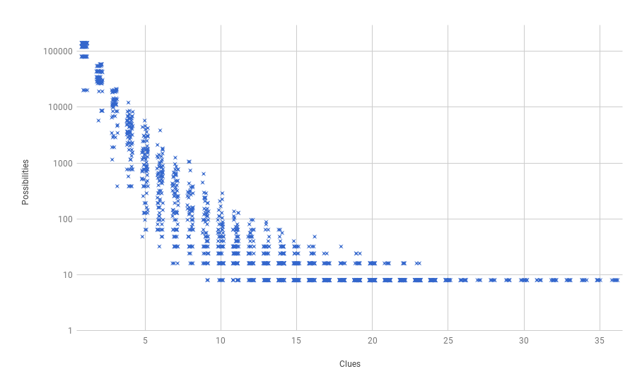
First, be aware that this is a semilogarithmic plot: The number of satisfactory solutions (“Possibilities”) on the y axis is shown on a logarithmic scale. Plotted on a linear scale, the whole thing is pretty much illegible.

Second, because there are so many samples which produce exactly the same number of possibilities, I’ve added a little jitter to the x axis to spread them out horizontally. Those dark little lines you see forming dashes across the bottom right of the chart are all results where there are exactly 8 solutions.

Here’s how I was wrong: Because of my many years of poking around in abstract combinatorial spaces and complex systems settings, I was convinced there would be a string “tipping point” when I first built this chart. That is, I figured that there would be a relatively slow drop in the number of “possibilities” for the first few additional clues added, and then all of a sudden a steep drop-off, and then relatively little gain made (if any) for the last few clues added.

That latter part is actually right, if you look at things. For this admittedly scant sample of (less than 2000 total) random trials, the last place I’ve ever found any “uncertainty” is when there are 23 clues. For all samples made of 24 or more clues, there’s complete certainty, and only eight satisfactory solutions remain out of all those \(362880\) possibilities.

But that doesn’t feel like it’s qualitatively similar to what’s happening on the left side. Here, we start shedding possibilities very quickly. Basically, for every clue you add, you’re seeing about half the possibilities disappear.

Third, notice, how spread out things get in the middle region. In part, this may be due to the combinatorics of randomly sampling from the set of clues: There are \(7140\) subsets with cluefulness = 3, \(58905\) with cluefulness = 4, and a whopping \(9075135300\) with cluefulness = 18. So the question may not be why it’s so “spread out” in the middle, but rather why it’s not very spread out by the time we get to cluefulness = 18 or so. By the time we reach that point, the vast majority of the samples are completly sufficient, though we still find a few with slight uncertainty.

The questions in hand

Now the original étude posed several questions, and after a couple of days of poking I’ve managed to at least get some insights into the first couple of questions posed.

One thing I asked: For a square of a given size, how many clues can I ignore and still eliminate all uncertainty about the labeling? Well, I have only managed to do this for a square of nine labels, but it looks like the answer is “a lot of them”. Seriously, I’d be pretty comfortable if you hid 10 of the 36 total clues from me. At least for a 3x3 square. That’s a third, basically. So it feels as if there’s a lot of redundant information in that collection of Manhattan distances, and that (for a square of this size, at least) things are a bit over-specified.

Another thing I asked: For a square of a given size, if I give you the best possible set of clues, how few might you need to be absolutely certain of the labeling? Here, things are a bit sketchier, because while I can glance at the chart and see where the best randomly-sampled subsets of constraints fall, I was in no sense trying to greedily add the best possible clues in a series of “steps”.

Which I might try, because it sounds like it may be useful.

That said, the first time I manage to see a completely-specified solution, we have 9 clues. This is such a sparse sampling, I wouldn’t be surprised at all if there were extreme cases over at 8 or even 7 clues. To be honest, there may well be very small subsets of clues. I just don’t have an intuition yet, except that I notice that the “empty” section of the lower left of this plot is really really tiny in comparison to the overall area covered.

Now I also asked some other questions.

First, of course, I haven’t really addressed the more salient aspect of just labeled squares: I said “for a square of a given size”, and this particular approach does a just-barely-feasible job for 3x3 squares. But the number of possible labelings of a 3x3 square is \(9! = 362880\); the number of possible labelings of a 4x4 square is \(16! = 20922789888000\). If my brute-force enumeration for one labeling takes about a minute on my laptop, then an enumeration for even one 4x4 labeling will take… \(57657600\) minutes, or close to 110 years. And since there are 120 pairs of labels for a 4x4 square, instead of 36 for a 3x3, multiply another four-fold just for fun.

So while this has been intriguing, and more than a little bit counterintuitive, perhaps the simplest thing that could possibly work isn’t going to “work” in the larger sense.

Listening to what the bad ideas can say

I’d like to better understand what’s happening in this “simple” little system of nine variables and 36 constraints.

Here are some intuitions and ideas I’ve had so far.

It seems clear to me that there are “better” and “worse” clues among the 36 Manhattan distances. That is, if I’m starting with zero clues and adding them, it seems as though (from the lower left margin of the cloud of sampled points) there is a small subset of clues I should select in order to drop towards certainty as fast as possible. But that sequence may be contingent on earlier choices, I admit. Since I framed the “adding clues” question in terms of a path, maybe I should consider what happens when (for example) I greedily add one clue at a time, picking the one that most reduces the number of possible labelings.

Similarly, looking at the upper right edge of the cloud of points, if I were forced to sequentially forget one clue at a time, it feels as though there is a greedy path I could take there as well. It may not be the case that every sequence of forgotten clues gets me to the “same place”, so this feels a bit trickier I admit. What is the overlap between the different subsets of 25 clues that produce complete confidence (reduce the possibilities to 8)? What’s the overlap, if any, among the 23-clue subsets that start to become less certain?

There is an important but implicit thing this exploration is yelling, too. As I noted above, there’s no way I could enumerate the absolute number of labelings for a 4x4 square, at least not using this simple-minded algorithm.

It seems there are two ways forward, then, since I do still want to understand what happens for 10x10 squares at least as well as I understand the case for 3x3 squares.

On the one hand, I could take a sampling approach. That is, instead of enumerating every possible labeling of a larger square, I could start sampling random labelings. The numbers are large enough that—as long as I can trust my sampling methods—I should at least start to get some hints of structure if there is any.

On the other hand, I could take a more first principles approach. For instance, in the current algorithm I’m actually building every possible labeling of the 3x3 square. It strikes me that there are probably smart-seeming ways to eliminate whole piles of those labelings as infeasible right away. For example, if the Manhattan distance between :x0 and :x1 is 1, then I need never build any configuration where that’s not the case. In other words, maybe “permutations of labels” isn’t quite the right representational approach to take here. Maybe something that starts from distances would be more effective.

And of course there may be possibilities for getting at things from both directions at the same time.

What I don’t want to do is construct a software library to handle this general class of problems. I may end up downloading something like a constraint-handling library to further explore, but the point of these études is not to “train” myself (and you) to download and run software, but rather to model simply-stated but difficult problems.

For example, here’s where I am right now.

Remember that I said my original intuition was that there would be a phase transition or “tipping point” in the number of possibilities vs the cluefulness. I’m not convinced yet that there won’t be, when we look at larger systems. This may be still such a small example that’s more like an “edge case”, where things haven’t had a chance to settle in yet. For example, there are more clues for larger squares, and more possible labelings, but the number of labelings is going up much faster than the number of Manhattan distance clues. For my desired “probably big enough” example of a 10x10 square, there are \(100! \approx 9.332622 \times 10^{157}\) possible labelings, and only \(4950\) clues. That said, the x axis in the 3x3 case is only 36 steps wide. Maybe the “tipping point” is already happening by the time we get to 1/36 clues, but may not have started happening at 1/4950.

Hopefully we’ll see.

And then there is the question of what happens when we “open up” the possible layouts: What about non-square rectangles? What about polyominoes? As I mentioned the other day, something odd happens when we move to polyominoes, since even a complete list of all the Manhattan distances is no longer sufficient to identify some small polyominoes. So there’s something “hidden” in my specification of a square, or a rectangle, or a polyomino arrangement of labels that is affecting how useful a “complete” set of Manhattan distance clues can be.

I wonder if the shape is itself a kind of constraint? After all, there are more rectangles of 3600 labels, compared to just the one 60x60 square. And there are a super huge number of 3600-block polyominoes.

I wonder if maybe a more general model that takes it into account would help understand things here? Again: hopefully we’ll see.

Oh, and

Here are the data I collected to draw that chart I showed you: