Watching the arithmetic sausage getting made
Draft of 2018.04.18
I’ve been making some slides for a talk I’ll give in a few weeks, and have been thinking a bit too much about ways of visualizing “what happens” when we do genetic programming. Most of the focus of the field is in the dynamics of search itself: folks visualize population diversities, and scores over time, and genealogies and pedigrees of various approximate solutions to the target problem. That’s a lot of stuff to see all at once, and as a rule when we do that sort of thing we’re prone to either seek out special cases that simplify the view, or collapse a lot of complicated data into summary statistics of some sort.
Lately my eyes have been wandering in a slightly different direction. Towards the dynamics of evaluation, rather than the “next level up” where learning and search happen.
I think I should make some notes. Let me back into this from a historical perspective: I’ll start by talking about “traditional tree-based GP” (the 30-year-old arithmetic symbolic regression stuff you’ll see if you glance at Wikipedia), then move a bit more towards the modern stack-based representations like Push, and then back the tour bus off the cliff into our destination: evaluating infinite programs.
Trees (gah, not again)
Let me steal my first example from the damned Wikipedia article:
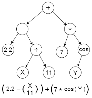
That is to say, the expression in question is \(f(x,y)=(2.2 - \frac{x}{11} + 7 \cos(y))\) when I typeset it in “traditional arithmetic” notation.
First, let me rewrite this expression in a lispier form, with the functions at heads of lists of arguments, by pulling the operators (including some implicit ones) to the fronts of some nested lists:
(+ (- 2.2 (/ x 11)) (* 7 (cos y)))
If you glance back at the diagram, you’ll see the root of the tree appears at the head of the expression (in this format), and the leaves of the tree are scattered down inside some nested parentheses.
Now if you’re the sort of person who likes to write Lisp or Clojure programs, this will be a familiar form. But as somebody who has—whether out of choice or academic obligations—been forced to write a program that evaluates this expression, you will know that when we “run” this “program” we’ll be keeping track of some intermediate values and partially-completed calculations along the way.
One way (surely not the only way) to evaluate this expression is to use a call stack-based calculator, which traces a depth-first path through the tree while maintaining the sense that it’s “done” when it “knows” specific values for each item on its frame stack. That is to say, something like this will happen:
+isn’t something we can evaluate yet, so create a new evaluation item and determine the value of its first argument,(- 2.2 (/ x 11))-isn’t something we can evaluate yet, so look at2.2- hey I know what
2.2is! that’s a number! push it on a stack though, because there’s more expression left /isn’t something we can evaluate yet, so…
and so forth.
As I say, this is one way to evaluate these tree-like expressions, but I imagine it’s one of the first we encounter. We start trying to evaluate a binary arithmetic operator but we find that some or both of its arguments aren’t simplified yet, so we dive into those and try to evaluate them, and so on recursively until we get to a leaf—which by the rules of syntax is either going to be a numerical constant or a variable reference like x or y.
But there are other ways to manipulate this structure and traverse it, without maintaining a collection of partially-completed evaluations. One approach is to transform the prefix-form nested expression into a more imperative postfix (reversePolish) order as:
infix:           (+ (- 2.2 (/ x 11)) (* 7 (cos y)))
becomes postfix: (2.2 x 11 / - 7 y cos * +)
To evaluate this stream of symbols, we’ll use a simple push-down stack for numbers we encounter or construct as we process each token in turn. If a token is a numerical constant, we’ll just push it to the stack. If it’s an operator like + or cos, we’ll pop its arguments from the stack (in what amounts to a reversed order, so that the RPN expression (2 1 -) can be read as “subtract 1 from 2”) and push the result back onto the stack. If the token is a variable, we’ll look up its value, and push that to the stack. And each step of the way, we’ll consume one more token from the RPN program, until we run out of tokens.
Say for example that I have assigned x to be 22 and y to be π. If we watch the implicit numerical stack here, it will do something like this on each step (if I write the top at the left):
[]          (2.2 x 11 / - 7 y cos * +) ; before we start, the stack is empty)
[2.2]       (x 11 / - 7 y cos * +)     ; 2.2 is a constant, so just push it
[22 2.2]    (11 / - 7 y cos * +)       ; x is a variable, so push its value
[11 22 2.2] (/ - 7 y cos * +)          ; another constant
[2 2.2]     (- 7 y cos * +)            ; divide 22/11 to make 2
[0.2]       (7 y cos * +)              ; subtract 2.2-2 to get 0.2
[7 0.2]     (y cos * +)                ; constant
[π 7 0.2]   (cos * +)                  ; variable
[-1 7 0.2]  (* +)                      ; cos(π) = -1
[-7 0.2]    (+)                        ; -1 * 7
[-6.8]      ()                         ; -7 + 0.2
And (hopefully, if I’ve done it right this time) \(-6.8\) is the “final answer” for the RPN expression (2.2 11 x / - 7 y cos * +), with those values assigned to x and y. And also the “final answer” for the equivalent prefix Clojure-like expression (+ (- 2.2 (/ x 11)) (* 7 (cos y))).
What we did and what we get
I honestly didn’t use an explicit (which is to say, conscious) algorithm to transform the original expression into infix form, and I didn’t use the shunting yard algorithm to convert that into RPN form. I just, you know, did it in my head. But such algorithms do exist, in case you’re wondering.
But notice that what we got by spending the effort.
First—and perhaps trivially, but I think not—one of the things that happened when I transformed the sort of loosey-goosey “traditional” expression \((2.2 - \frac{x}{11} + 7 \cos(y))\) into the prefix formatted (+ (- 2.2 (/ x 11)) (* 7 (cos y))) was that a lot more parentheses appeared. Those parentheses arose because I explicitly set off each sub-expression as either an explicit constant or variable, or else as a list containing a function and all its arguments. And also along the way I also paid attention to non-commutative functions, like - and /.
To evaluate this form, though, I think—perhaps by habit—that I will need a call stack and a bunch of nested recursive stuff. By transforming the expression into Art Burks’s RPN format like this (2.2 x 11 / - 7 y cos * +), I’ve traded the call stack for a value stack. That is, I maintain intermediate values as I process the overall expression, rather than juggling a stack of intermediate expressions. The two are no doubt exactly equivalent in theory, but in some visceral sense the former delays the gratification I receive as soon as I have an actual number in hand.
One more thing, which may not be something we “got” but which is definitely something I’m here to “give” you: Notice that the result is on top of the number stack when we’ve finished calculating (2.2 x 11 / - 7 y cos * +). We’ve reduced the expression to the equivalent expression (-6.8).
But notice that we have that stack with numerical values on it—sometimes it’s empty, but not often—from the very beginning. And that every stack along the way has a top value. We move through the series of stacks ([], [2.2], [22 2.2], [11 22 2.2], [2 2.2], [0.2], [7 0.2], [π 7 0.2], [-1 7 0.2], [-7 0.2], [-6.8]). The top number on the stack in each step follows the “path” \((\varnothing,2.2,22,11,2,0.2,7,\pi,-1,-7,-6.8)\), where I’ve used \(“\varnothing”\) to represent “no number”.
I want to come back to that series, next time.
Getting pushy
I’ve spent a lot of time (in other essays) talking about the Push language—and am trying desperately to finish a draft of an overview of the whole language—so I won’t spend much time on it here. There’s one facet of Push’s behavior I want to invoke, and bring to this analysis of evaluation.
Push calls its operators “instructions”. There are far more instructions in even a trivial implementation of Push than we’ve been using here, but they all work more or less the same way as our RPN arithmetic instructions work. That is, when the Push instruction that’s equivalent to our + operator is evaluated, two arguments are popped from the stack, their sum is calculated, and that result is pushed onto the stack. In Push, “the stack” I’m referring to with respect to adding numbers is specifically one that holds numbers (there are others).
But there’s one more salient aspect of Push instructions that I want to bring over: Whenever a Push instruction is executed, it first determines whether all its arguments are present on the stack(s). If they are, then it pops those arguments and pushes the result(s), just like we’re doing here in this arithmetic toy. But if the arguments are not all present, the instruction is ignored: even if some of the arguments are present, they are left where they sit, and nothing happens1 except that the instruction is passed over.
This permits a very interesting sort of robustness in Push programs.
Let’s look at our RPN friend (2.2 x 11 / - 7 y cos * +) again. If you look at the stack trace I presented above, you’ll see that in every step where an operator (instruction) is executed, there were enough items on the stack to satisfy the requirements. When / is processed, there are already two numbers on the stack to be its arguments. When cos is processed, there is at least one number on the stack.
Because we started from a traditional, syntactically-familiar arithmetic expression like \(f(x,y)=(2.2 - \frac{x}{11} + 7 \cos(y))\), and because I was kinda careful transforming that into a prefix and RPN form, it just happens to be true that there are always enough arguments for each operator as we walk along the sequence (2.2 x 11 / - 7 y cos * +).
What happens when there aren’t enough arguments, though? Suppose we try removing that initial 2.2 from the program, giving us (x 11 / - 7 y cos * +)
[]       (x 11 / - 7 y cos * +)
[22]     (11 / - 7 y cos * +)
[11 22]  (/ - 7 y cos * +)
[2]      (- 7 y cos * +)        ; missing arguments, nothing happens
[2]      (7 y cos * +)
[7 2]    (y cos * +)
[π 7 2]  (cos * +)
[-1 7 2] (* +)
[-7 2]   (+)
[-5]     ()
Well, that’s interesting. As long I am willing to “forgive” missing arguments in this way, the reduced program still “worked”—in the sense of passing through the point where in a traditional interpreter or compiler there would have been a syntax error. As a result, the function this reduced RPN expression represents is no longer \(f(x,y)=(2.2 - \frac{x}{11} + 7 \cos(y))\), but turns out to be something more like \(g(x,y)=(\frac{x}{11} + 7 \cos(y))\).
Not only has the initial constant 2.2 disappeared, but the silent failure of the subtraction operator has changed the sign of the second term. In some sense, there is still a valid expression, since there’s a number present on the stack when we’re done.
What happens if I delete the last token from the RPN program, giving me (2.2 x 11 / - 7 y cos *)?
[]          (2.2 x 11 / - 7 y cos *)
[2.2]       (x 11 / - 7 y cos *)
[22 2.2]    (11 / - 7 y cos *)
[11 22 2.2] (/ - 7 y cos *)
[2 2.2]     (- 7 y cos *)
[0.2]       (7 y cos *)
[7 0.2]     (y cos *)
[π 7 0.2]   (cos *)
[-1 7 0.2]  (*)
[-7 0.2]    ()
We seem to still be “good”, in the sense that there is always a number around when we expect one, even though in the end there are more than one “result” items left on the number stack. You might be tempted to interpret this RPN program as representing one that “returns” two results from these inputs, but let’s leave notion that aside for another day. For now, let me follow the approach I used with the “proper” and undamaged RPN expression, and say that the top number on the stack at the end of the calculation—the point where I have evaluated every token in the program—is the “returned” value.
The “answer” is now -7, in other words.
So maybe we can say, for this reduced expression, that we’re “evaluating” some different algebraic expression, which looks more like \(f_1(x,y)=7 \cos(y)\). But that doesn’t feel quite right, since most of the time and effort was spent doing the work to calculate that other component, \(f_2(x,y)=(2.2 - \frac{x}{11})\), but we ended up “throwing it away”—in the sense that it’s left being the second number on our stack, and therefore doesn’t interact with the first.
That seems a bit weird. Yes, there is some number on the top of the stack in each step. And yes, when we evaluate the original “complete” tree’s expression, (2.2 x 11 / - 7 y cos * +), we might want to think we’re “moving towards” the “final answer” at each step. In the intact RPN expression, we’re traversing the syntactically-complete arithemtic tree in a particular order, accumulating intermediate values along the way, until we reach the root node + and “return” the overarching sum of all the terms.
But as soon as I deleted a term from (2.2 x 11 / - 7 y cos * +), I was doing something subtly different. In the case where I dropped the first 2.2, we “skipped” a subtraction operator and got a different answer. In the case where I dropped the final +, we “skipped” another operator, but this time ended up with… well, “two” answers.
The linearized RPN version (2.2 x 11 / - 7 y cos * +), coupled with the Push rule “skip operators that lack arguments”, no longer seems the be quite the same thing as (+ (- 2.2 (/ x 11)) (* 7 (cos y))). In the case where I’ve deleted the final token, it’s as though we’ve combined two different expressions, and shuffled their calculation together into a single dynamic process. If another + token were to come along later, then maybe we’d recombine them. But as long as we stop with (2.2 x 11 / - 7 y cos *) (lacking that last +), we have done work on the two still-independent “calculations” of \(f_1(x,y)=7 \cos(y)\) and \(f_2(x,y)=(2.2 - \frac{x}{11})\).
The top number on the stack is, in some sense, a “step towards” a final result. But only insofar as it’s the result of some combining operator farther along the way….
A few more pokes and prods
What happens if I “run” an RPN program twice, consecutively?
[]               (2.2 x 11 / - 7 y cos * + 2.2 x 11 / - 7 y cos * +)
[2.2]            (x 11 / - 7 y cos * + 2.2 x 11 / - 7 y cos * +)
[22 2.2]         (11 / - 7 y cos * + 2.2 x 11 / - 7 y cos * +)
[11 22 2.2]      (/ - 7 y cos * + 2.2 x 11 / - 7 y cos * +)
[2 2.2]          (- 7 y cos * + 2.2 x 11 / - 7 y cos * +)
[0.2]            (7 y cos * + 2.2 x 11 / - 7 y cos * +)
[7 0.2]          (y cos * + 2.2 x 11 / - 7 y cos * +)
[π 7 0.2]        (cos * + 2.2 x 11 / - 7 y cos * +)
[-1 7 0.2]       (* + 2.2 x 11 / - 7 y cos * +)
[-7 0.2]         (+ 2.2 x 11 / - 7 y cos * +)
[-6.8]           (2.2 x 11 / - 7 y cos * +)
[2.2 -6.8]       (x 11 / - 7 y cos * +) ;; start over
[22 2.2 -6.8]    (11 / - 7 y cos * +)
[11 22 2.2 -6.8] (/ - 7 y cos * +)
[2 2.2 -6.8]     (- 7 y cos * +)
[0.2 -6.8]       (7 y cos * +)
[7 0.2 -6.8]     (y cos * +)
[π 7 0.2 -6.8]   (cos * +)
[-1 7 0.2 -6.8]  (* +)
[-7 0.2 -6.8]    (+)
[-6.8 -6.8]      ()
So concatenating two copies of an RPN program like this works… well, I can only bring myself to say “as expected”, algorithmically. The doubled program no longer seems to represent the algebraic function \(f(x,y)=(2.2 - \frac{x}{11} + 7 \cos(y))\), but rather something weird, like “\(f(x,y)\) twice”. One is tempted to say this final stack [-6.8 -6.8] is some kind of “vector” of two independent calculations, right?
Now let me try this concatenation out with the truncated RPN expression (x 11 / - 7 y cos * +) (lacking the initial constant). Remember, this is the one where we invoked the Push “silent failure” rule, when we were missing arguments.
[]         (x 11 / - 7 y cos * + x 11 / - 7 y cos * +)
[22]       (11 / - 7 y cos * + x 11 / - 7 y cos * +)
[11 22]    (/ - 7 y cos * + x 11 / - 7 y cos * +)
[2]        (- 7 y cos * + x 11 / - 7 y cos * +)
[2]        (7 y cos * + x 11 / - 7 y cos * +) ;; failed subtraction
[7 2]      (y cos * + x 11 / - 7 y cos * +)
[π 7 2]    (cos * + x 11 / - 7 y cos * +)
[-1 7 2]   (* + x 11 / - 7 y cos * +)
[-7 2]     (+ x 11 / - 7 y cos * +)
[-5]       (x 11 / - 7 y cos * +)
[22 -5]    (11 / - 7 y cos * +)
[11 22 -5] (/ - 7 y cos * +)
[2 -5]     (- 7 y cos * +)  ;; subtraction does not fail
[-7]       (7 y cos * +)
[7 -7]     (y cos * +)
[π 7 -7]   (cos * +)
[-1 7 -7]  (* +)
[-7 -7]    (+)
[-14]      ()
As expected, the first time we encounter the - operator, we lack an argument and fail silently. But as we proceed through the program a second time, we’ve left “residue” on the stack from the earlier pass through, and so on the subsequent pass through, we do have two argument for subtraction.
I find myself wondering what will happen if I “keep going”. Well, this is a memoryless process, and there’s no reason I can’t just slap another copy of the (reduced) RPN program into the right hand side of my hand-made interpreter now.
[-14]       (x 11 / - 7 y cos * +)
[22 -14]    (11 / - 7 y cos * +)
[11 22 -14] (/ - 7 y cos * +)
[2 -14]     (- 7 y cos * +)
[-16]       (7 y cos * +)  ;; subtraction works again
[7 -16]     (y cos * +)
[π 7 -16]   (cos * +)
[-1 7 -16]  (* +)
[-7 -16]    (+)
[-23]       ()
I could keep going, if I simply dropped another copy of (x 11 / - 7 y cos * +) into the slot. What do you think would happen over time?
We seem to be counting down by increments of 9, don’t we? That is, after finishing each series of (x 11 / - 7 y cos * +) tokens, the number on the top of the stack is reduced by nine.
But the number on the top of the stack at other times is not necessarily reduced by nine. Most of the other values appear in each loop of this execution, don’t they? I see π whenever I’ve executed the token y, and I see 11 whenever that appears as a constant in the program being run.
Suppose ask you the obvious question: What would happen if we kept re-stocking the program with copies of (x 11 / - 7 y cos * +) forever? Every ninth step, a new number nine lower than the last one would appear, so you might be tempted to say that the “result” is tending towards “negative infinity”.
What would happen if instead of cycling through the reduced program, we cycled through the “intact” one, (2.2 x 11 / - 7 y cos * +)? In that case, an additional copy of a number will appear. The stack will keep growing, but the value on top will remain the same in each loop.
a wee bit of abstraction
Let me work through one more of my examples by hand: The case where we dropped the last token, (2.2 x 11 / - 7 y cos *). When I ran this, above, you’ll recall I ended up with two values on the stack. When I now execute it twice in succession, I get a stack of four values: two copies of the same pair.
[]                 (2.2 x 11 / - 7 y cos * 2.2 x 11 / - 7 y cos *)
[2.2]              (x 11 / - 7 y cos * 2.2 x 11 / - 7 y cos *)
[22 2.2]           (11 / - 7 y cos * 2.2 x 11 / - 7 y cos *)
[11 22 2.2]        (/ - 7 y cos * 2.2 x 11 / - 7 y cos *)
[2 2.2]            (- 7 y cos * 2.2 x 11 / - 7 y cos *)
[0.2]              (7 y cos * 2.2 x 11 / - 7 y cos *)
[7 0.2]            (y cos * 2.2 x 11 / - 7 y cos *)
[π 7 0.2]          (cos * 2.2 x 11 / - 7 y cos *)
[-1 7 0.2]         (* 2.2 x 11 / - 7 y cos *)
[-7 0.2]           (2.2 x 11 / - 7 y cos *)
[2.2 -7 0.2]       (x 11 / - 7 y cos *)
[22 2.2 -7 0.2]    (11 / - 7 y cos *)
[11 22 2.2 -7 0.2] (/ - 7 y cos *)
[2 2.2 -7 0.2]     (- 7 y cos *)
[0.2 -7 0.2]       (7 y cos *)
[7 0.2 -7 0.2]     (y cos *)
[π 7 0.2 -7 0.2]   (cos *)
[-1 7 0.2 -7 0.2]  (*)
[-7 0.2 -7 0.2]    ()
Every time I run (2.2 x 11 / - 7 y cos *), the net result is that I add a new copy of the pair [-7 0.2] to the stack. Those values depend on the arguments x and y, but they seem to be constant as long as x and y are constant.
Suppose I were to abstract the sequence of tokens 2.2 x 11 / - 7 y cos * as Y. Whenever I invoke Y in my interpreter now, I will now just push the pair -7 0.2 onto the stack all at once, and not bother consuming anything from the number stack at all.
[]              (2.2 x 11 / - 7 y cos * 2.2 x 11 / - 7 y cos *)
[]              (Y 2.2 x 11 / - 7 y cos *)
[-7 0.2]        (2.2 x 11 / - 7 y cos *)
[-7 0.2]        (Y)
[-7 0.2 -7 0.2] ()
Can I do the same thing for the other examples? Sure. Suppose I say the intact program (2.2 x 11 / - 7 y cos * +) is represented by X, and know that its result is -6.8. Instead of substituting beforehand, let me make the change in-line, as though the “interpreter” was “recognizing” the pattern as it executed the code….
[]          (2.2 x 11 / - 7 y cos * + 2.2 x 11 / - 7 y cos * +)
[]          (X 2.2 x 11 / - 7 y cos * +)
[6.8]       (2.2 x 11 / - 7 y cos * +)
[6.8]       (X)
[-6.8 -6.8] ()
What about (x 11 / - 7 y cos * +)? Say this is Z. But notice that it doesn’t feel “self-contained” in the same way as our X and Y did. If I run Z with “no arguments” (an empty stack), I “get a result” of -5. If there is an “argument” available, then I end up subtracting nine from that value.
[]    (x 11 / - 7 y cos * + x 11 / - 7 y cos * +)
[]    (Z x 11 / - 7 y cos * +)
[-5]  (x 11 / - 7 y cos * +)
[-5]  (Z)
[-14] ()
Those three abstractions, though….
X: (2.2 x 11 / - 7 y cos * +)   => push -6.8
Y: (2.2 x 11 / - 7 y cos *  )   => push the pair -7 0.2
Z: (    x 11 / - 7 y cos * +)   => push -5 if stack is empty, or subtract 9
There’s an odd sort of mathematical relationship between X and Y and Z, isn’t there? I mean, as ordered collections of tokens they contain one another—in the sense that X contains the source code of both Y and Z, and that each of those contain much of one another’s source code. But they’re not doing quite the same things.
Isn’t that weird?
[That’s a leading question]
But of course, this is all happening when the arguments x and y are fixed. These RPN programs are, after all, supposed to represent “functions” of some sort. What kind of functions are X and Y and Z, in this scheme? How do they relate to one another
a bit more abstraction
I’m suddenly concerned that by only looking at fixed assignments to the variables x and y in my programs, I’m masking something interesting.
I don’t actually need to do that here. I can deal with the abstract variables I have in hand.
Let me work out what’s happening with my little program again, but this time without knocking down the argument variables to specific values. I’ll start with the “full function”, which I’ve called X above, and use traditional arithmetic expressions on the stack instead of the explicit values.
[]                        (2.2 x 11 / - 7 y cos * +)
[2.2]                     (x 11 / - 7 y cos * +)
[x 2.2]                   (11 / - 7 y cos * +)
[11 x 2.2]                (/ - 7 y cos * +)
[(x÷11) 2.2]              (- 7 y cos * +)
[(2.2-(x÷11))]            (7 y cos * +)
[7 (2.2-(x÷11))]          (y cos * +)
[y 7 (2.2-(x÷11))]        (cos * +)
[cos(y) 7 (2.2-(x÷11))]   (* +)
[(7*cos(y)) (2.2-(x÷11))] (+)
[(2.2-(x÷11)+7*cos(y))]   ()
That wasn’t so bad. What about my truncated function Y?
[]                        (2.2 x 11 / - 7 y cos *)
[2.2]                     (x 11 / - 7 y cos *)
[x 2.2]                   (11 / - 7 y cos *)
[11 x 2.2]                (/ - 7 y cos *)
[(x÷11) 2.2]              (- 7 y cos *)
[(2.2-(x÷11))]            (7 y cos *)
[7 (2.2-(x÷11))]          (y cos *)
[y 7 (2.2-(x÷11))]        (cos *)
[cos(y) 7 (2.2-(x÷11))]   (*)
[(7*cos(y)) (2.2-(x÷11))] ()
Well of course it’s the same as the first several steps of X. It simply lacks the final + to stitch things together. What about Z?
[]                  (x 11 / - 7 y cos * +)
[x]                 (11 / - 7 y cos * +)
[11 x]              (/ - 7 y cos * +)
[(x÷11)]            (- 7 y cos * +)
[(x÷11)]            (7 y cos * +) ;; nope
[7 (x÷11)]          (y cos * +)
[y 7 (x÷11)]        (cos * +)
[cos(y) 7 (x÷11)]   (* +)
[(7*cos(y)) (x÷11)] (+)
[(x÷11)+(7*cos(y))] ()
Recall that we’re not experiencing a failure when we encounter an operator that lacks one or more arguments, and we’re also not currying the function. We’re simply skipping the operator entirely, as though it were a NOOP. So where I’ve labeled nope in the trace of Z, a - token lacks an argument; there is only one number on the stack at that point.
what if?
As I glance at the RPN program (2.2 x 11 / - 7 y cos * +), I notice there are ten tokens in it: three numerical constants, two variables, four binary operators and one unary operator (cos).
So far I’ve only been looking at what happens when I delete a single token from one end of X, and repeat those variations. In doing so, I’ve noticed that in some cases the repeated code can just be slapped into the “code stack” and executed after it’s been emptied, but in other cases (the one I’ve called Z) there is a difference in behavior when the program is run the first time (giving -5), and all subsequent times (subtracting nine).
And we’ve seen how the difference between the first and later iterations of Z arise because (unlike Y, which has also had a single token removed) is somehow because the first iteration “wants” something that doesn’t appear on the stack. Later iterations leave items on the stack, and that same operator (executed later) doesn’t fail. Instead, it “reaches back” into the leftover results of earlier iterations.
Meanwhile, variant Y leaves two items on the stack in each iteration—including the first one. Somehow, both of those “answers” are self-contained, at least within the scope of Y. One “chunk” produces (2.2-(x÷11)) and another “chunk” produces (7*cos(y)). Indeed, I could say that Y is a concatenation of two different little self-contained programs F1 = (2.2 x 11 / -) and F2 = (), where F1 consumes no arguments and produces (2.2-(x÷11)) and F2 consumes no arguments and produces (7*cos(y)), couldn’t I?
[]                        (2.2 x 11 / - 7 y cos *)
[]                        (F1 7 y cos *)
[(2.2-(x÷11))]            (7 y cos *)
[(2.2-(x÷11))]            (F2)
[(7*cos(y)) (2.2-(x÷11))] ()
That bit about “consumes no arguments” seems salient somehow. The chunk of code I’ve called Z does “consume arguments”, in the sense that it contains a - instruction that “wants” an argument that isn’t present when the number stack is empty. It’s “reaching left” into the results of some earlier calculation, right?
To “square up” Z, in the sense that it stops having any failing instructions in it, I’d just need to add something “to the left”, which leaves one (or more) items on the stack. That could be a constant, or a variable… or indeed it could be anything at all that doesn’t itself “want” for an input or argument. So any self-contained block of RPN code could appear there, of any size at all.
Let’s insert some arbitrary self-contained bit of code, P and see what happens to Z. Note that P by definition takes no “arguments” from the stack (in the same way X and Y consume no items), and produces one or more items. P could be a simple constant, or a collection of smaller self-contained blocks, or even an infinite collection of such blocks. Without loss of generality, let me say P produces one or more (possibly infinite number) products \(p_{-1}\) and \(p_{-2}\) and so on:
[]                                    (P x 11 / - 7 y cos * +)
[p[-1] p[-2] …]                       (x 11 / - 7 y cos * +)
[x p[-1] p[-2] …]                     (11 / - 7 y cos * +)
[11 x p[-1] p[-2] …]                  (/ - 7 y cos * +)
[(x÷11) p[-1] p[-2] …]                (- 7 y cos * +)
[(p[-1]-(x÷11)) p[-2] …]              (7 y cos * +)
[7 (p[-1]-(x÷11)) p[-2] …]            (y cos * +)
[y 7 (p[-1]-(x÷11)) p[-2] …]          (cos * +)
[cos(y) 7 (p[-1]-(x÷11)) p[-2] …]     (* +)
[(7*cos(y)) (p[-1]-(x÷11)) p[-2] …]   (+)
[((p[-1]-(x÷11))+(7*cos(y))) p[-2] …] ()
Think of P as the context in which Z is being executed. It’s the stuff that already exists on the stack, into which Z (or any code) can reach for its arguments.
We can consider the “needs” of arbitrary RPN code, not just X and Y (which have no “needs” because they’re self-contained blocks) or Z (which “needs” one item from the stack to avoid a failed operator), but any sequence of constants, variables and operators at all.
For instance, what about (+ + + *)? This is just a sequence of four binary operators, each of which “wants” two inputs, but all of which can produce one output as well. Let me do the trick with prepending P again, adding additional terms down the stack to compensate for missing arguments:
[] (P + + + *)
[p[-1] p[-2] p[-3] p[-4] …] (+ + + *)
[(p[-2]+p[-1]) p[-3] p[-4] …] (+ + *)
[(p[-3]+p[-2]+p[-1]) p[-4] …] (+ *)
[(p[-4]+p[-3]+p[-2]+p[-1]) p[-5] …] (*)
[p[-5]*(p[-4]+p[-3]+p[-2]+p[-1]) p[-6 ]…] ()
We can avoid any failed operations in (+ + + *) by prepending five items on the stack.
Note though that (+ + + *) is perfectly reasonably code to run, as long as Push rule for missing arguments is in place. It’s not syntactically incorrect, but if we run it in isolation (with nothing on the stack) we’ll end up with an empty stack in the end, too. Being “self-contained” in the sense I’ve been using it means that no arguments would be consumed, if they were present, not that no items are consumed or produced when no items are present.
It’s about the past, in other words.
Stitching an infinite arithmetic scarf
I want to close this up now, because we’ve got something lovely to talk about next time. So far, I’ve talked about taking arithmetic expressions, and transforming them into postfix RPN expressions. Then I talked about the special “Push rule for missing arguments”, which permits silent failure of arbitrary RPN “code” whenever an argument is missing for an operator. I noticed that in the example “program” X we started with, I could still run it (thanks to the rule) whenever I deleted the first or last tokens, though the behavior of Y (deleting the last token) was somehow different from the behavior of Z. Specifically, when I ran concatenated copies of X and Y and Z, the latter was “weird” because it somehow “reached back” into its own stack’s history for missing arguments, whereas X could be “compressed” into a single self-contained “token” of its own that produced a specific single value whenever it was invoked, and Y could be considered as a pair F1 and F2.
Finally, we talked a bit about what makes Z weird, and how it “reaches back” to gather arguments from its own history. I pushed this farther by looking at that weird block (+ + + *), which “reached back” for five arguments it “needed” to run.
Somehow, it may have come across that having added the “Push rule” so I could run arbitrary code with an empty stack, I am now throwing stuff back onto the stack to make the “Push rule” unnecessary. Yes, but also no.
What I want to talk to you about next time is infinite programs.
Let’s try an experiment.
Remember that I said above: there are ten tokens in our X program? That is: three constants, two variable references, four binary operators and one unary operator.
Suppose we write those onto a 10-sided die, and roll the die a lot of times. A huge number of times, even. Actually let me make a slight substitution, because it’ll be useful next time: let’s say that instead of the constants \(2.2\) and \(11\) and \(7\) we inherited from the Wikipedia example, we have three arbitrary constants \(k_1\), \(k_2\) and \(k_3\).
So here’s the markings on the face of the 10-sided die: (k_1, x, k_2, /, -, k_3, y, cos, *, +). Roll that die a lot of times, and think of the sequence of results you get as a “really big program” in RPN syntax.
Say you produce \(N\) items this way. Here’s an example I just made with a simple script:
(/ cos y + + k_1 * x * x / k_1 * x k_1 x y cos y k_2 x x + x / + / + + * + * k_1 k_2 * k_3 + / k_1 k_3 / + k_2 y k_1 / k_3 / * k_1 k_2 * cos k_3 x * cos x cos k_2 / - k_3 y cos k_3 y / cos y * x k_3 * + * cos* y - - x + - x cos k_2 - * - / + cos x cos k_2 cos cos cos x k_1 - * + - k_3 cos + y + - k_3 / k_3 k_1 + k_3 / y - k_2)
Do one for yourself. Make it as long as you think you need.
How many “self-contained blocks” are there?
I’ve spent a little time working through my random sample for the first few steps by hand, using the P trick from above to “reach back” for non-existent arguments as needed. I’ve also added a little :: notation to better separate the number stack (on the left) from the program being run (on the right, in parentheses).
[] :: (P / cos y + + k_1 * x * x / k_1 * x k_1 x y cos y k_2 x x + …)
[p[-1] …] :: (/ cos y + + k_1 * x * x / k_1 * x k_1 x y cos y k_2 x x + …)
[(p[-2]÷p[-1]) p[-3] …] :: (cos y + + k_1 * x * x / k_1 * x k_1 x y cos y k_2 x x + …)
[cos(p[-2]÷p[-1]) p[-3] …] :: (y + + k_1 * x * x / k_1 * x k_1 x y cos y k_2 x x + …)
[y cos(p[-2]÷p[-1]) p[-3] …] :: (+ + k_1 * x * x / k_1 * x k_1 x y cos y k_2 x x + …)
[(cos(p[-2]÷p[-1])+y) p[-3] …] :: (+ k_1 * x * x / k_1 * x k_1 x y cos y k_2 x x + …)
[(p[-3]+(cos(p[-2]÷p[-1])+y)) p[-4] …] :: (k_1 * x * x / k_1 * x k_1 x y cos y k_2 x x + …)
[k_1 (p[-3]+(cos(p[-2]÷p[-1])+y)) p[-4] …] :: (* x * x / k_1 * x k_1 x y cos y k_2 x x + …)
[((p[-3]+(cos(p[-2]÷p[-1])+y))*k_1) p[-4] …] :: (x * x / k_1 * x k_1 x y cos y k_2 x x + …)
[x ((p[-3]+(cos(p[-2]÷p[-1])+y))*k_1) p[-4] …] :: (* x / k_1 * x k_1 x y cos y k_2 x x + …)
[(((p[-3]+(cos(p[-2]÷p[-1])+y))*k_1)*x) p[-4] …] :: (/ k_1 * x k_1 x y cos y k_2 x x + …)
[(p[-4]÷(((p[-3]+(cos(p[-2]÷p[-1])+y))*k_1)*x)) p[-5] …] :: (k_1 * x k_1 x y cos y k_2 x x + …)
[k_1 (p[-4]÷(((p[-3]+(cos(p[-2]÷p[-1])+y))*k_1)*x)) p[-5] …] :: (* x k_1 x y cos y k_2 x x + …)
[((p[-4]÷(((p[-3]+(cos(p[-2]÷p[-1])+y))*k_1)*x))*k_1) p[-5] …] :: (x k_1 x y cos y k_2 x x + …)
[x ((p[-4]÷(((p[-3]+(cos(p[-2]÷p[-1])+y))*k_1)*x))*k_1) p[-5] …] :: (k_1 x y cos y k_2 x x + …)
[k_1 x ((p[-4]÷(((p[-3]+(cos(p[-2]÷p[-1])+y))*k_1)*x))*k_1) p[-5] …] :: (x y cos y k_2 x x + …)
[x k_1 x ((p[-4]÷(((p[-3]+(cos(p[-2]÷p[-1])+y))*k_1)*x))*k_1) p[-5] …] :: (y cos y k_2 x x + …)
[y x k_1 x ((p[-4]÷(((p[-3]+(cos(p[-2]÷p[-1])+y))*k_1)*x))*k_1) p[-5] …] :: (cos y k_2 x x + …)
[cos(y) x k_1 x ((p[-4]÷(((p[-3]+(cos(p[-2]÷p[-1])+y))*k_1)*x))*k_1) p[-5] …] :: (y k_2 x x + …)
[y cos(y) x k_1 x ((p[-4]÷(((p[-3]+(cos(p[-2]÷p[-1])+y))*k_1)*x))*k_1) p[-5] …] :: (k_2 x x + …)
[k_2 y cos(y) x k_1 x ((p[-4]÷(((p[-3]+(cos(p[-2]÷p[-1])+y))*k_1)*x))*k_1) p[-5] …] :: (x x + …)
[x k_2 y cos(y) x k_1 x ((p[-4]÷(((p[-3]+(cos(p[-2]÷p[-1])+y))*k_1)*x))*k_1) p[-5] …] :: (x + …)
[(x+x) k_2 y cos(y) x k_1 x ((p[-4]÷(((p[-3]+(cos(p[-2]÷p[-1])+y))*k_1)*x))*k_1) p[-5] …] :: (…)
For a long time, it feels as though each step wants to “reach back” farther into the pre-existing P values for arguments. But then a string of variables and constants comes along, and it feels as though we’re safely working in a separate block. The value p[-5] sits there on the nominal bottom of the stack for a long time.
Is it safe, though? As we move farther through the program, sometimes we’re adding new things to the stack from the program directly—the constants, or the variable references—and sometimes we’re consuming two arguments to produce one result (the binary operators).
Meanwhile, the top item on the stack is getting remarkably ornate, isn’t it? By the time I got bored, it was (p[-4]÷(((p[-3]+(cos(p[-2]÷p[-1])+y))*k_1)*x))*k_1), which is (if I’ve done the work correctly)
Admittedly much of this is just peppering constants, so it might be somewhat simpler in principle (for instance, by cancelling the \(k_1\) terms in the outer numerator and denominator). But at the same time, realize that the \(p_{-i}\) terms are what I’ve called “self-contained blocks”, but that doesn’t mean they’re constants. In fact, in this context it seems as though they may be functions of \(x\) and \(y\) in their own right.
Every time we reach a stretch of constants and variable references like (… x k_1 x y …) we seem to be decreasing the probability that some later operator will come along and have to reach back into P for a missing argument. It seems that, if only we could get enough of those self-contained single-item blocks onto the stack, we’d be “safe”.
Similarly, every time we encounter a stretch of code like (… / + / + + * + * …) (which you’ll notice I stopped before I reached in the sample I made), I start to worry than any surplus stuff we have on the stack will be exhausted and I’ll need to “reach back” even further into P for arguments. There’s nothing wrong with doing that, of course. It’s just that it feels a bit like a strange sort of balance, doesn’t it?
In the current 10-sided die I told you to use, the three constants and two variables produce a net increase of one stack item when the interpreter encounters them. The operator cos has no net effect, since it consumes and produces one item. The four binary operators consume two items each, and produce only one, for a net reduction of one. Whenever any of those four operators appears in a program at the start, it will by necessity “reach back” for \(p_{-1}\) and \(p_{-2}\). Whenever one appears in the second position in a program, it will also “reach back” for at least one argument—depending on the previous token—because none of our ten tokens produce more than one item at a time.
If we happened to have started our random RPN program like this:
(k_3 k_2 k_1 y k_1 k_2 k_1 y k_2 k_1 x …)
then it would take a string of ten or more binary operators to exhaust the bounty of stuff on the stack. Each of those eleven tokens is itself a “self-contained block”, in the sense I’ve described. If I roll the ten-sided die now to determine the next token, there’s a \(\frac{1}{10}\) chance that we get cos, a \(\frac{5}{10}\) chance we get a constant or variable reference, and a \(\frac{4}{10}\) chance we “reach back” into this stack (which now has [x k_1 …] on its top) with a binary operator.
If the program is infinite, then while there’s always a chance that a series of binary operators will wear away the sand-pile of pre-existing self-contained blocks on the stack, the larger that sack of self-contained blocks becomes, the less likely that seems.
So maybe we can talk about the expected size for these self-contained blocks, in an infinite-in-both-directions program.
How big would that be?
-
In Klapaucius, what actually happens is that an
:erroris the result of any instruction lacking arguments, which is pushed to the:errorstack. But that’s not important here. ↩