Arithmetic sausage links
Draft of 2018.04.23
Last time I spent some time talking about the ways we might “unroll” an arithmetic expression, starting from traditional mathematical notation and ending up in RPN format: First, into something like the prefix notation of Lisp languages—where the operator appears first, followed by its arguments. Then into something closer to RPN notation—where the operator appears after its arguments have been pushed onto a stack, so they can be consumed by subsequent operators and replaced by the products of those operations. Finally we talked a bit about the Push language’s “leave it alone” rule (for lack of a better name), which states that whenever an operator (“instruction”, in Push) appears, but there are missing arguments it “wants” that aren’t present on the stack, we ignore the operator and move along instead of “crashing”.
I made a point of saying that it’s not an error in Push for an operator to be applied even when it lacks one or more arguments. Then I spent some time talking about what happens in the process of executing a Push-like RPN arithmetic “program”.
We watched the program get consumed, token by token, while new values appeared on the numerical stack. Constant values were pushed directly from the program’s “head” onto the stack, variable references from the program pushed their values to the stack, and operators consumed items from the stack (if present) and pushed results back onto that same stack.
Finally, I spent some time talking about how many arguments these Push-like programs “want” but can’t have, which is a thing that seems to happen most when they begin running. Since we continue processing even when an operator lacks arguments, I suggested we provide a sort of abstract “preimage” P, representing “stuff already on the number stack”, which can “hand over” self-contained code blocks that represent definite but abstract values.
Throughout this arc, I walked through programs by writing either the values or the expressions for each item on the number stack, as I walked through the tokens in the RPN program one by one. The simple example I stole from the Wikipedia page on
genetic programming was \(f(x,y)=(2.2 - \frac{x}{11} + 7 \cos(y))\), which is something like (2.2 x 11 / - 7 y cos * +) in an RPN form, and when I write the expressions for each item in the stack (on the square brackets on the left) and the remaining program tokens in the parentheses on the right, we pass through these steps:
STACK                     PROGRAM

[]                        (2.2 x 11 / - 7 y cos * +)
[2.2]                     (x 11 / - 7 y cos * +)
[x 2.2]                   (11 / - 7 y cos * +)
[11 x 2.2]                (/ - 7 y cos * +)
[(x÷11) 2.2]              (- 7 y cos * +)
[(2.2-(x÷11))]            (7 y cos * +)
[7 (2.2-(x÷11))]          (y cos * +)
[y 7 (2.2-(x÷11))]        (cos * +)
[cos(y) 7 (2.2-(x÷11))]   (* +)
[(7*cos(y)) (2.2-(x÷11))] (+)
[(2.2-(x÷11)+7*cos(y))]   ()
Thus, starting from an empty stack at the beginning of the process, we can watch the RPN form get converted—unsurprisingly, I hope—into something that looks a lot like \(f(x,y)=(2.2 - \frac{x}{11} + 7 \cos(y))\). But that’s written in “traditional” infix format.
Then I compared that trace to the execution of the program block (+ + + *), executed using the “preimage” P approach I mentioned. That is, whenever any operator “needs more” arguments, it can reach down into the infinite collection of “stuff already on hand” P and obtain those arguments at will.
STACK                                     PROGRAM

[]                                        (P + + + *)
[p[-1] p[-2] p[-3] p[-4] …]               (+ + + *)
[(p[-2]+p[-1]) p[-3] p[-4] …]             (+ + *)
[(p[-3]+p[-2]+p[-1]) p[-4] …]             (+ *)
[(p[-4]+p[-3]+p[-2]+p[-1]) p[-5] …]       (*)
[p[-5]*(p[-4]+p[-3]+p[-2]+p[-1]) p[-6 ]…] ()
Note how the code blocks (2.2 x 11 / - 7 y cos * +) and (+ + + *) act somewhat differently. As I run (2.2 x 11 / - 7 y cos * +), there are no steps where it “wants” to reach back into P for “missing arguments”. It is in some sense a self-contained block of code, for which every operator has all the necessary arguments already on hand. When I run it, the number of new items placed on the stack is balanced by the number of arguments consumed by operators later on. On the other hand, (+ + + *) doesn’t contain any arguments (no constants, no variable references), and therefore it “wants” to grab five items from P before it finally produces the “self-contained” block p[-5]*(p[-4]+p[-3]+p[-2]+p[-1]) on the stack.
There is something interesting going on here, though, because in each step, the “thing” (expression, or value) I’ve pushed onto the stack is itself one of these “self-contained blocks”. Even though the code remaining to be executed may later demand arguments not present, the items on the stack have each, in themselves, been “balanced”.
This led me to ask about the relative “sizes” of the stack items, as opposed to the code block being “run”.
So here’s the markings on the face of the 10-sided die: (
k_1,x,k_2,/,-,k_3,y,cos,*,+). Roll that die a lot of times, and think of the sequence of results you get as a “really big program” in RPN syntax.Say you produce \(N\) items this way. Here’s an example I just made with a simple script:
(/ cos y + + k_1 * x * x / k_1 * x k_1 x y cos y k_2 x x + x / + / + + * + * k_1 k_2 * k_3 + / k_1 k_3 / + k_2 y k_1 / k_3 / * k_1 k_2 * cos k_3 x * cos x cos k_2 / - k_3 y cos k_3 y / cos y * x k_3 * + * cos* y - - x + - x cos k_2 - * - / + cos x cos k_2 cos cos cos x k_1 - * + - k_3 cos + y + - k_3 / k_3 k_1 + k_3 / y - k_2)Do one for yourself. Make it as long as you think you need.
How many “self-contained blocks” are there?
After I asked that question, I of course spent a good deal of time thinking about it myself. It turns out that I may have been misleading both of us with a strange notational quirk.
Let’s fix that now.
Full circle
One interesting thing about this arc is the glibness with which I’ve been shifting between representation schemes. In some sense, all of the programs and “self-contained blocks” and traditional equations and prefix and postfix programs are “the same thing”, aren’t they? But sometimes I write “traditional” infix format like (x÷11), sometimes I write the numerical value (given some assigned x value), and sometimes—at least on the “program” side—I write RPN code like (11 x /).
Nonetheless, because of habit? assumptions? subconscious sadism? I chose to represent my “self-contained blocks” on the stacks using traditional arithmetic syntax:
STACK                     PROGRAM

[]                        (2.2 x 11 / - 7 y cos * +)
[2.2]                     (x 11 / - 7 y cos * +)
[x 2.2]                   (11 / - 7 y cos * +)
[11 x 2.2]                (/ - 7 y cos * +)
[(x÷11) 2.2]              (- 7 y cos * +)
[(2.2-(x÷11))]            (7 y cos * +)
[7 (2.2-(x÷11))]          (y cos * +)
[y 7 (2.2-(x÷11))]        (cos * +)
[cos(y) 7 (2.2-(x÷11))]   (* +)
[(7*cos(y)) (2.2-(x÷11))] (+)
[(2.2-(x÷11)+7*cos(y))]   ()
I mean seriously, what even is (2.2-(x÷11))? We recognize it from familiarity, but asking “how big is it?” is problematic. But. But! Look at what happens if, instead of writing those traditional infix forms, I instead write more RPN code on the stack side. Watch closely, as I add a little semantic sugar in the form of parentheses around each individual item I push to the stack:
STACK                        PROGRAM

[]                           (2.2 x 11 / - 7 y cos * +)
[(2.2)]                      (x 11 / - 7 y cos * +)
[(x) (2.2)]                  (11 / - 7 y cos * +)
[(11) (x) (2.2)]             (/ - 7 y cos * +)
[(x 11 /) (2.2)]             (- 7 y cos * +)
[(2.2 x 11 / -)]             (7 y cos * +)
[(7) (2.2 x 11 / -)]         (y cos * +)
[(y) (7) (2.2 x 11 / -)]     (cos * +)
[(y cos) (7) (2.2 x 11 / -)] (* +)
[(7 y cos *) (2.2 x 11 / -)] (+)
[(2.2 x 11 / - 7 y cos * +)] ()
Isn’t that lovely? Notice that I’ve moved the program from the right hand side, to the left hand side, where now it appears in exactly the same format as it was on the right. Sure looks like I’ve done a lot of work for absolutely no reason whatsoever!
Well, no. I did something more, didn’t I?
Maybe this fragment of code might be interesting, extracted from the long random sample I provided above:
STACK                                                    PROGRAM
[]                                                       (P k_2 y k_1 / k_3 / * k_1 k_2 * cos k_3 x * …)
[(P)]                                                    (k_2 y k_1 / k_3 / * k_1 k_2 * cos k_3 x * …)
[(k_2) (P)]                                              (y k_1 / k_3 / * k_1 k_2 * cos k_3 x * …)
[(y) (k_2) (P)]                                          (k_1 / k_3 / * k_1 k_2 * cos k_3 x * …)
[(k_1) (y) (k_2) (P)]                                    (/ k_3 / * k_1 k_2 * cos k_3 x * …)
[(y k_1 /) (k_2) (P)]                                    (k_3 / * k_1 k_2 * cos k_3 x * …)
[(k_3) (y k_1 /) (k_2) (P)]                              (/ * k_1 k_2 * cos k_3 x * …)
[(y k_1 / k_3 /) (k_2) (P)]                              (* k_1 k_2 * cos k_3 x * …)
[(k_2 y k_1 / k_3 / *) (P)]                              (k_1 k_2 * cos k_3 x * …)
[(k_1) (k_2 y k_1 / k_3 / *) (P)]                        (k_2 * cos k_3 x * …)
[(k_2) (k_1) (k_2 y k_1 / k_3 / *) (P)]                  (k_2 * cos k_3 x * …)
[(k_1 k_2 *) (k_2 y k_1 / k_3 / *) (P)]                  (cos k_3 x * …)
[(k_1 k_2 * cos) (k_2 y k_1 / k_3 / *) (P)]              (k_3 x * …)
[(k_3) (k_1 k_2 * cos) (k_2 y k_1 / k_3 / *) (P)]        (x * …)
[(x) (k_3) (k_1 k_2 * cos) (k_2 y k_1 / k_3 / *) (P)]    (* …)
[(k_3 x *) (k_1 k_2 * cos) (k_2 y k_1 / k_3 / *) (P)] (…)
Perhaps you can see what I’m seeing if you focus on the last few steps:
[(k_1 k_2 *) (k_2 y k_1 / k_3 / *) (P)]                  (cos k_3 x * …)
[(k_1 k_2 * cos) (k_2 y k_1 / k_3 / *) (P)]              (k_3 x * …)
[(k_3) (k_1 k_2 * cos) (k_2 y k_1 / k_3 / *) (P)]        (x * …)
[(x) (k_3) (k_1 k_2 * cos) (k_2 y k_1 / k_3 / *) (P)]    (* …)
[(k_3 x *) () (k_1 k_2 * cos) (k_2 y k_1 / k_3 / *) (P)] (…)
Both the constant k_3 and the variable reference x gets pushed onto the stack as their own self-contained blocks. Then the operator * multiplies the top two items on the stack, and we say that it “pops the top two items and pushes their product” whenever we explain Push-like languages.
But in fact, in this notation what the binary operator * does can also be described as (1) append itself to the top item on the stack, and (2) prepend the second item on the stack to that. In other words, the binary * “means” both “multiplication” and also something like
If the top item on the stack is
A, and the second itemB, and the operatorC, then delete the top two items on the stack and replace with the single itemBAC: the concatenation of their RPN string representations.
Similarly, the unary operator cos also “means” something like this:
Append the operator to the top item on the stack.
Things have become a matter of something a lot more like string manipulation, at least for these arithmetic operations.
A simpler problem
I had asked what you might expect to happen to the sizes of the items on the stack, as you evaluated an infinite sequence of uniform random sample from the set of tokens in the Wikipedia example. That is, the “program” you’d produce by rolling a die labeled (k_1, x, k_2, /, -, k_3, y, cos, *, +).
But using this new approach, where we treat the unary and binary operators as string-manipulating-and-concatenating ones, you might find it simpler to count the number of tokens in each item on the stack.
If you evaluate an infinite program composed of (k_1, x, k_2, /, -, k_3, y, cos, *, +) in uniform proportions, but keep the RPN representations of each intermediate item on the stack, the question becomes: How many tokens will be in each item on the stack, after a long long time?
Whenever you encounter a token like k_1 or x, you add a totally new “self-contained block” to the stack, and it will contain one token.
Whenever you encounter a unary operator like cos, you modify the top thing on the stack to make a new one which is just the original item, with the new token appended. You increment the size of the top item by one.
Whenever you encounter a binary operator like + or /, you consume the top two items on the stack but then can easily construct the result by string concatenation. The result will therefore contain all the tokens from the two argument items, plus one for the new operator you append.
The results of these string manipulations are still composed of tokens. What do you expect the distribution of the number of tokens to be like?
Looking to see
I spent some time yesterday writing a simple Ruby program to look and see. Here’s a part of it:
tokens = ['k_1', 'x', 'k_2', '/', '-', 'k_3', 'y', 'cos', '*', '+']
stack  = ["k_4"] * 10

def frequencies( array )
  hash = Hash.new(0)
  array.each{|key| hash[key] += 1}
  hash
end

10000.times do |step|
  item = tokens.sample
  case item
  when /k_\d/
    stack.unshift item
  when "x","y"
    stack.unshift item
  when "cos"
    arg = stack.shift
    stack.unshift (arg + " " + item)
  when "+", "*", "/", "-"
    arg1 = stack.shift
    arg2 = stack.shift
    stack.unshift [arg2,arg1,item].join(" ")
  else
    stack = stack
  end
  # puts stack.inspect
  # puts stack.count
end

sizes = stack.collect {|i| i.split(" ").count}
puts frequencies(sizes).inspect
In the first two lines, I simply state the ten “tokens” from the open question as strings, and prepare a stack with a rather artificial preimage of items already on it. I used "k_4" here just to be sure to see when things came from the preimage as opposed to the “program” being run, but with a little more effort I might have differentiated the items. I didn’t think that was salient.
Then I define a simple frequencies method that counts the number of each unique item in an arbitrary array. Later, I’ll use this to count the frequencies of the sizes of each item in the stack.
Then we do the thing: I sample a new random tokens item, and depending on which one I manipulate the (string) contents of the stack, as I described above. In each loop, one more (random) token from the “program” is being processed, and something is happening on the top items of the stack.
You may notice some commented-out reporting statements in there. You might want to look into what happens there, out of curiosity, if they’re uncommented—that’s what I did.
Finally, I take the stack and count the number of tokens in each string, by splitting each string on whitespace and counting the number of components. Then I report the frequencies of those “sizes”.
When I run this code, I get something like this:
{1=>494,
 11=>7,
 2=>52,
 3=>77,
 58=>1,
 39=>2,
 10=>8,
 22=>7,
 29=>4,
 33=>2,
 220=>1,
 42=>2,
 8=>21,
 7=>17,
 5=>46,
 12=>7,
 19=>7,
 17=>6,
 6=>15,
 14=>10,
 23=>3,
 25=>2,
 15=>10,
 13=>4,
 4=>26,
 9=>11,
 21=>4,
 351=>1,
 18=>11,
 50=>2,
 64=>1,
 209=>1,
 32=>2,
 26=>2,
 80=>1,
 116=>1,
 63=>2,
 271=>1,
 41=>1,
 54=>2,
 67=>1,
 38=>1,
 60=>2,
 215=>1,
 31=>4,
 40=>2,
 37=>3,
 47=>4,
 109=>1,
 30=>3,
 92=>1,
 49=>1,
 120=>2,
 119=>1,
 27=>2,
 56=>2,
 118=>1,
 28=>1,
 105=>1,
 36=>2,
 75=>1,
 24=>3,
 190=>1,
 77=>1,
 34=>1,
 62=>1,
 224=>1,
 51=>1,
 16=>3,
 185=>1,
 165=>1,
 45=>1,
 46=>1,
 35=>3,
 144=>1,
 358=>1,
 146=>1,
 76=>1,
 182=>1,
 221=>1,
 53=>1,
 52=>2}
That’s in an arbitrary order, because we’re adding a new key-value pair whenever our count of the tokens in each item on the stack encounters a new number. If I plot these values (manually, because I’m lazy), maybe you’ll find it more useful:
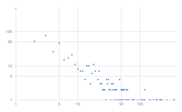
I’ve gone ahead and presented this on a log-log plot, where the horizontal axis is the number of tokens in an item, and the vertical axis the number of items on the stack with that many tokens. It may look vaguely familiar from somewhere, but it seems a bit noisy. Let me do the same thing, but for a million “program tokens” executed sequentially instead of a mere ten thousand:
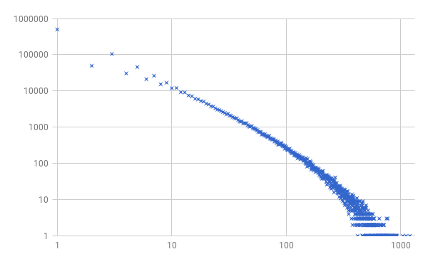
Well, well. That’s rather pretty, isn’t it?
Let’s leave the inevitable Complexological discussion of what distribution this seems to be for another day. Whether it’s log-normal, power law, or a double Pareto distribution—all somewhat questionable, since there are discrete changes in size here, and very particular probabilities because of the “10-sided die” we’re using to generate these “programs”—we can see that there are a lot of 1-token items, and very few items with loads of tokens. But there are in fact some items that are really frickin’ huge. The largest observed was well over 1000 tokens long.
Indeed: While it may be very rare, the longer one goes with this uniform random process, the more likely it seems that a binary operator will be applied to two even larger items on the stack. The probabilities may be low for such events, but they do seem to be feasible. It feels likely that there’s no real upper limit on the size of an item on the stack, doesn’t it?
By the same token (heh), we’re spending what feels like a lot of time fiddling with innumerable copies of (x) and (k_2) and so on. The vast majority of the little stuff—the ones with few tokens—are probably all accounted for in early steps of the process. We’ve surely got every combination of {x,y,k_1,k_2,k_3} and "+" after a million random steps, for example: (x x +) and (x y +) and so forth.
I wonder how many of each thing we end up with?
stack item          observed number on stack
"k_3"             : 10032
"y"               : 10023
"k_1"             : 10020
"x"               : 10011
"k_2"             : 9879

"k_1 cos"         : 994
"y cos"           : 992
"x cos"           : 983
"k_2 cos"         : 960
"k_3 cos"         : 959

"k_1 k_1 +"       : 127
"k_2 y /"         : 124
"k_2 k_2 *"       : 120
"x y -"           : 120
"k_3 y +"         : 119
"k_1 k_3 *"       : 116
"k_3 y -"         : 116
"y x /"           : 116
"k_1 k_1 *"       : 115
"y x +"           : 115
"x y *"           : 114
"y k_1 *"         : 114
"k_3 k_3 -"       : 114
"k_1 y *"         : 114
"k_2 k_3 +"       : 113
"y k_2 /"         : 113
"k_1 k_2 -"       : 112
"k_2 k_2 /"       : 112
"y y /"           : 111
"y k_1 +"         : 111
"k_3 k_1 +"       : 111
"x k_1 +"         : 110
"k_2 cos cos"     : 109
"k_1 x -"         : 109
"x x +"           : 108
"k_1 k_2 /"       : 108
"y y *"           : 107
"x k_3 -"         : 107
"k_3 k_3 /"       : 106
"y k_1 -"         : 106
"y k_3 -"         : 106
"k_3 x +"         : 106
"k_1 x *"         : 105
"x y /"           : 105
"x x /"           : 105
"k_1 k_3 +"       : 104
"k_3 k_1 *"       : 104
"k_2 k_1 *"       : 104
"k_2 x /"         : 103
"x x -"           : 103
"k_2 x +"         : 103
"k_2 k_2 +"       : 103
"k_2 y *"         : 103
"y k_3 +"         : 103
"k_1 x +"         : 102
"k_3 k_3 *"       : 102
"y x -"           : 102
"y k_1 /"         : 102
"k_3 k_2 -"       : 102
"k_1 cos cos"     : 102
"x cos cos"       : 101
"x k_1 /"         : 101
"y y +"           : 101
"x y +"           : 100
"k_1 y /"         : 100
"k_2 k_1 -"       : 99
"y k_3 /"         : 99
"k_2 k_3 *"       : 98
"k_3 y /"         : 98
"k_2 y +"         : 98
"k_3 k_1 -"       : 98
"k_2 y -"         : 98
"x k_3 /"         : 97
"k_1 x /"         : 97
"x k_3 +"         : 96
"k_3 k_2 /"       : 96
"k_3 k_3 +"       : 96
"k_1 y +"         : 96
"k_1 k_1 -"       : 96
"k_2 k_1 /"       : 95
"x k_2 /"         : 95
"x k_3 *"         : 95
"k_2 x *"         : 94
"k_2 k_1 +"       : 94
"k_3 cos cos"     : 94
"k_1 k_3 /"       : 94
"k_3 x -"         : 93
"y k_2 +"         : 93
"x k_2 *"         : 93
"y x *"           : 93
"k_3 x *"         : 93
"y y -"           : 92
"k_3 y *"         : 91
"k_1 k_2 *"       : 91
"y k_2 -"         : 90
"y k_2 *"         : 90
"k_3 k_2 *"       : 89
"k_1 y -"         : 89
"k_1 k_2 +"       : 89
"x k_1 -"         : 89
"x x *"           : 88
"y k_3 *"         : 88
"k_3 x /"         : 87
"k_2 x -"         : 87
"x k_2 +"         : 87
"k_1 k_3 -"       : 87
"k_2 k_2 -"       : 86
"k_2 k_3 -"       : 86
"x k_1 *"         : 86
"k_2 k_3 /"       : 86
"k_3 k_2 +"       : 84
"x k_2 -"         : 83
"k_3 k_1 /"       : 80
"y cos cos"       : 78
"k_1 k_1 /"       : 76

"k_3 x - cos"     : 19
"y x / cos"       : 19
"x x cos -"       : 19
"x y * cos"       : 19
"k_1 cos k_1 +"   : 18
"k_1 k_1 cos /"   : 18
"k_3 cos k_1 /"   : 17
"k_3 cos y *"     : 17
"k_3 cos k_1 +"   : 17
"k_2 k_3 + cos"   : 17
"y x cos -"       : 17
"x cos k_1 -"     : 17
"k_3 cos cos cos" : 17
"k_1 k_2 cos *"   : 17
"y cos x /"       : 17
"k_2 k_1 * cos"   : 16
"y cos k_2 -"     : 16
...
And so on. That’s just the result of running frequencies(stack), with some sorting afterwards, and it’s only the most frequently-occurring items here. There were on the order of a hundred thousand total (non-unique) items on the stack in this run I processed for this table, after walking through 1000000 tokens of the “program” to form the RPN expressions on the stack.
Interestingly (but again, not surprisingly, given the plot of size frequencies I showed above), the “average” size of an item on the stack is about ten tokens, if we just divide the number of items created into the number of tokens processed. But the vast majority of those have size 1, and so there’s a lot of room for larger, more ornate (and often “baroque”) expressions to crop up as single-copy items.
Therefore, many of the items on the stack are (1) very large and much more complicated than the frequent and simple ones I’ve shown here, and (2) they were mainly only present as single copies out of ten thousand or so “samples”. Neither of those observations should be surprising, but I find them noteworthy.
“Random guessing”, at least in the case of Push-like RPN code, seems to produce a lot of little useless junk, and only a few larger self-contained expressions.
In the next step of this arc, we’ll come back to that observation. I’ll take the time to look at the frequency of different behavior of these various self-contained block strings. That is, how often do (x y +) and (y x +) (which are I suppose semantically identical?) show up, vs (x y -) and (y x -)? There’s an open question (for me) about what rules might apply for simplifying RPN expressions to check that, but at a minimum we could just look at a bunch of input:output pairs as evidence of similarity or difference.
Why bother?
One of the things we tend to do when we’re building genetic programming systems is begin with random code. “Random code” in the old tree-based representation days was usually “random binary trees”, especially when working with arithmetic expressions like the ones I’m discussing here. In our work with stack-based schemes like Push, we tend to just pick random collections of uniformly-sampled tokens (and, in Push, some block-like structure which isn’t salient here).
There’s an interesting difference between constructing a single tree by filling it with random branches and leaves, and building a random RPN program by stringing together random tokens. In the former case, there is always “one answer”—one root of the tree, which by convention “is” the “returned value” of the tree. In the latter case, where we are building and consolidating (and in some cases, breaking back down) a series of tree-like structures on the runtime stacks, we need to rely on an additional convention like “the answer is the top thing on the stack when we quit.”
Many of us working in stack-based representations find this rather liberating. There are a lot of awkward-feeling things you need to be willing to do when you exchange chunks of type-correct S-expression trees, that you don’t need to do when you exchange chunks of RPN-style sequential “programs”. For instance, Push handles the question of type safety by simply pushing items of various types to type-specific stacks. So where I’ve been showing you RPN code involving numbers and numerical operators, we could also have (mixed into the same programs) boolean literals, variables and operators. During execution, we’d use type-checking at runtime to sort items onto the correct stacks, and to acquire arguments for operators.
It all works out.
But the cost (if in fact it is a cost) of running an arbitrary sequence of tokens and saying “the last item on top of the [specific] stack is the answer” at the end is shown in the work I’ve shared here. When I run a block of a million tokens drawn from my (arguably) very reasonable 10-sided die, we end up with nearly a hundred thousand items on the stack. We get some final item on top of the stack, at every step. But the vast majority of the things pushed there are buried beneath a subsequent pile of later arrivals.
Since the program being run is random—not different from the typical genetic programming practice for initialization—how can we justify that “extra work” done in calculating all those earlier steps, which are subsequently ignored?
Might there be a “better” answer somewhere half-way down the stack, rather than in the arbitrarily-specified top-position-at-exactly-N-steps?
How much work are we doing along the way?
Now I suspect some colleagues of the Push-using variety would be thinking, “Hey, nobody would be stupid enough to run a hundred-thousand token random program! We run a thousand hundred-token random programs, instead! Also, why am I made out of straw?” So yes: I’m saying (and showing, I think) that even a hundred-token program in this teeny little abbreviated toy 10-token world produces a remarkable number of individual self-contained blocks along the way. Imagine running a thousand hundred-token programs, in sequence… divided by a token that empties the stack. There. Now you have a single hundred-thousand-and-a-few-more token program, and you’re running it.
You’re just, by my argument, enforcing the places where you construct self-contained items on the stack. And (I will argue), almost none of your 100-token random programs will leave only a single item on the stack at the end of the run.
But this is the kicker: What if we treat these earlier, typically ignored early calculations as “draft answers”? When I run a random 100-token program, I actually get thirty separate items on the stack, sorted here by frequency:
count : block
6     : "k_4"
5     : "y"
2     : "k_1"
2     : "x"
1     : "y x -"
1     : "k_2"
1     : "k_1 x -"
1     : "k_3 k_3 x - +"
1     : "k_3"
1     : "x x *"
1     : "y x - cos"
1     : "k_3 y *"
1     : "y cos"
1     : "k_1 k_3 k_3 / * k_2 - cos x *"
1     : "k_4 k_4 k_4 k_4 + / +"
1     : "k_3 y k_3 k_1 / k_3 x - - k_2 / k_3 k_3 - y k_2 * / - * y - /"
1     : "y x *"
1     : "y k_1 k_1 y y / - k_3 * / * x / k_1 cos x * / x + k_1 -"
1     : "y k_1 cos * cos"
I’m not saying that this 100-token program “includes” or “represents” or “is”—at least in any useful sense—“six copies” of the program (k_4)… but when you run it, it sure looks like it does. It also includes/represents/is a whole bunch of other structurally- and functionally-diverse stuff. I have no more justification to expect the self-contained item that happened to be on top of the stack—the one-token item (k_3) in this case—to be the “right answer”, than I do (y k_1 k_1 y y / - k_3 * / * x / k_1 cos x * / x + k_1 -)—which was third on the stack.
Indeed, I’m much more likely to think of the big long expression (y k_1 k_1 y y / - k_3 * / * x / k_1 cos x * / x + k_1 -) as somehow being a “better candidate” as a model of some target function, compared with \(f(x,y) = k_3\) or \(f(x,y) = y\) or even \(f(x,y) = k_1+\frac{k_2}{k_3}\). At least if, you know… I’m trying to make these programs do something interesting.
I’ll talk about that next time. For now, wonder: How many functionally distinct items will I expect to see on my stack, after running a million steps from my 10-sided die?